On This Page
Google Sheets for SEO
So I love Google Sheets and use it daily for my work as an SEO. I wanted to share the top 15 Google Sheets formulas and features I use to shave hours off my work week and make my life easier. Keep in mind all of these features are in Google Sheets. No need to download any add-ons.
Keep in mind Google Sheets doesn’t do well with large tables. You can learn more about Google Sheets limits here: https://support.google.com/drive/answer/37603?hl=en.
Personally, I notice that I start having issues with Google Sheets freezing or crashing when I use over 20k rows.
Highlight Duplicates
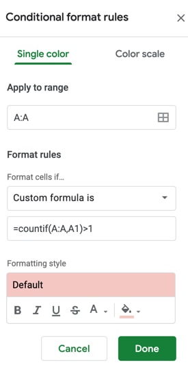
In Google Sheets, you can only remove duplicates. You can’t “find” them. But there’s a quick hack you can use to highlight all duplicates in a column. It’s very simple.
- Select the entire column that you want to check for duplicates.
- In the Google Sheets menu click on “Format” and then “Conditional formatting”.
- Under “Format rules” choose “Custom formula is”.
- In the “Value of formula” field add
=COUNTIF(A:A,A1)>1- This formula will look for duplicates in all cells of column A. If you need to look for duplicates in another column, simply change all the “A”s in the formula to that column letter. Example:
=COUNTIF(B:B,B1)>1
- This formula will look for duplicates in all cells of column A. If you need to look for duplicates in another column, simply change all the “A”s in the formula to that column letter. Example:
- Under the “Formatting style” choose a color. I used red.
- Then click “Done”.
Google Sheets Example + Template
IMPORTXML
In Google Sheets you can pull in the page title, meta description and H1 for a URL in a matter of seconds.
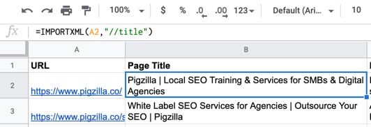
Page Title
=IMPORTXML("URL GOES HERE","//title")Meta Description
=IMPORTXML("URL GOES HERE","//meta[@name='description']/@content")H1
=IMPORTXML("URL GOES HERE","//h1")Google Sheets Example + Template

TRANSPOSE
Sometimes you have a table of data that you’d like to flip around. You can use the TRANSPOSE function to do this.
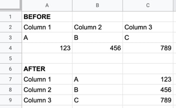
=TRANSPOSE(RANGE)Google Sheets Example + Template
VLOOKUP
VLOOKUP is an amazing way to find and match up data in a Google Sheet. VLOOKUP can be a little tricky so let me explain how it works first. You can look for a value in a certain range and return the data next to it. For example, let’s say you have two tabs. In one tab you have a list of URLs with their page titles and meta descriptions. In the other tab you have a list of URLs and their impression and click data from Google Search Console. You can use VLOOKUP to match up data from both tabs.
So here’s how you use it. In the second table that you will be searching in, the first column that you select in the range needs to match the type of data you are looking up. For example, if you are looking up a URL from the first tab, the first column that you select in the range needs to have the URLs in them. You can only return data from any columns to the right of this column. So you will need to arrange your data first before using VLOOKUP.
Let’s try it out. Type in =VLOOKUP then select the cell you want to look up data for. Next, choose the range you want to search for it in. Then enter the number for the column that you want to return the data from in the range. After that type in “false” and hit enter.
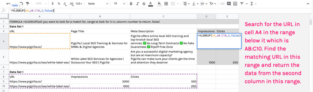
=VLOOKUP(LOOKUP VALUE,RANGE,CULUMN # TO RETURN,false)Google Sheets Example + Template
Split Text to Columns
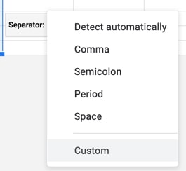
Select the cell or columns you want to split. In the Google Sheets menu click on “Data” and then “Split text to columns”. A small box will pop up that says “Separator”. Choose “Custom” Here you can choose where you want to split the data.
You can split the following URL at these different points:
https://www.pigzilla.co/articles/tracking-convertkit-forms-with-google-analytics-tag-manager/
- “://” to split the protocol from the domain.
- “.co” to get only the URL slug.
- “www.” to split the subdomain from the domain.
- “/articles” to split the parent folder from the page path.
Keep in mind, the cells that you split will not remain intact. I recommend copying the original cells and splitting the text on the copied cells that way you still have the originals. Also, when the data is split, it will replace any data in the cells to the right of it so make sure you don’t have any important data to the right.
Google Sheets Example + Template
CONCATENATE
There are many times where you need to merge data. For example, one cell contains the word “Bob” and another one contains “Smith”. You can use CONCATENATE to merge these two cells into a new cell that says “Bob Smith”.
I use the CONCATENATE formula to create URLs in bulk. These can be used for creating redirects in bulk or to create new URLs when moving to a new domain. I also use it to write page titles and meta descriptions at scale.
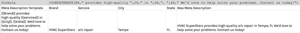
You can choose cells to consolidate. You can also insert words and phrases if needed. To insert words or phrases use quotes and make sure to include necessary spaces in the quotes. Example ” Words Go Here “.
=CONCATENATE(A1,A2)=CONCATENATE(A1," Words Go Here "A2)Google Sheets Example + Template
Mystery Match
Haha, ok so this formula is not called mystery match but I don’t know what it’s called. I use it to see if canonicals are self-referencing. You can use it for anything though. It simply tells you if the data in two cell match each other.
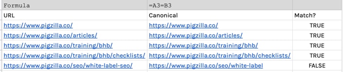
If the two cells match, it will return “TRUE”. If they don’t match it will return “FALSE”.
=A2=B2You can also use the IF function to customize this a bit more. You can choose what it will return if there’s a match or not.
=IF(A2=B2,"Match","No Match")Google Sheets Example + Template
Convert Letter Case
I’ve had instances of website data that was in all caps that I needed to make lowercase. You can use the LOWER function to make all the letters lowercase. Other useful options are UPPER which makes all letters uppercase and PROPER which makes only the first letter of each word uppercase.
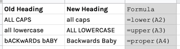
=UPPER(A1)=LOWER(A1)=PROPER(A1)Google Sheets Example + Template
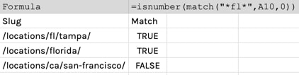
MATCH
I use the MATCH function to see if a cell contains a certain word. Let’s say I have a list of page titles and I want to know which ones mention the word “florida”. Or URLs that have “fl” in them.
If you are looking for an exact word to match simply put it in quotes like the formula below.
=ISNUMBER(MATCH("florida",A3,0))If you are looking for a partial match you would add asterisks like the formula below. This means you are looking for those letters in that order but they can have any characters before or after them.
=ISNUMBER(MATCH("*fl*",A3,0))This formula would find both of these URLs as a match because they both contain “fl” in them:
- /locations/fl/orlando/
- /locations/florida/
Google Sheets Example + Template
REGEXMATCH
You can also use REGEXMATCH to see if a cell contains any of several words.
I like to look for test pages, paid landing pages and conversion pages that need to either be removed or made non-indexable. I’ll check to see if any of them contain the words “test”, “thank you”, “confirmation” or “lp”.
=REGEXMATCH(A12,"thank|test|confirm|lp")Google Sheets Example + Template
Go Deeper: https://www.youtube.com/watch?v=BHApCQHu98g
Trim
Sometimes you have data that has a space before or after it like so:
” lorem ipsum”
“lorem ipsum ”
You can use the TRIM function you can remove this empty space in a jiffy!
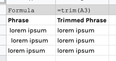
=TRIM(A3)Google Sheets Example + Template
Go Deeper: https://support.google.com/docs/answer/3094140?hl=en
LEN
When writing page titles and meta descriptions I like to make sure they are not over the recommended character limit per SEO best practices. For this I use LEN.
The LEN function will count the number of characters in a cell for you.
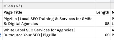
=LEN(A2)Google Sheets Example + Template
Go Deeper: https://support.google.com/docs/answer/3094081?hl=en
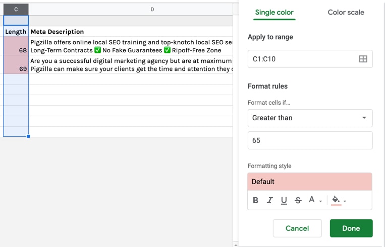
Conditional Formatting
But I take this a step further with conditional formatting. I like to have any page titles and meta descriptions over a certain length turn red. You can do this by:
-
- Select the entire Length column that you want to turn red if it’s over a certain length.
- In the Google Sheets menu click on “Format” and then “Conditional formatting”.
- Under “Format rules” choose “Greater than”.
- In the “Value of formula” field enter the maximum number of characters you’d like the cell to be.
- Under the “Formatting style” choose a color. I used red.
- Then click “Done”.
Google Sheets Example + Template
COUNTA
I use COUNTA to count the number of cells that are not blank. This can be used for many different reasons. I’ve used this to create a summary tab in SEO audits that show how many issues total were discovered.
=COUNTA(A3:A10)Google Sheets Example + Template
Go Deeper: https://productivityspot.com/count-non-blank-cells-google-sheets/
Query Function
I saved the best for last! Let’s say you have a big table of data you’ve exported from a tool like Screaming Frog or Ahrefs. You can choose to pull in only some of this data into another tab in order to analyze it.
Here’s how the formula looks:
=QUERY('TAB NAME'!RANGE:RANGE,"select COLUMN LETTER, COLUMN LETTER",1)I use the QUERY function to review backlink profiles, perform content audits and check for overlapping keywords in Google Search Console. For example, let’s say you’ve exported all the data from the “Internal” tab in Screaming Frog. It would look like this: Sample Data
You can use the QUERY function to pull in only Columns A and C using the formula below.
=QUERY('Screaming Frog Export'!A:EV,"select A, C",1)You can also include the WHERE function to only include certain pieces of data. You can use this QUERY and WHERE function to pull in only Columns A and C if the content in column B says “text/html; charset=UTF-8.
=QUERY('Screaming Frog Export'!A:EV,"select A, C WHERE B = 'text/html; charset=UTF-8'",1)Go Deeper: https://www.benlcollins.com/spreadsheets/google-sheets-query-sql/
Google Sheets Example + Template
Whew!
That was a lot to cover. But it wasn’t even the tip of the iceberg so keep exploring Google Sheets. I hope you find some of these functions useful. 🙂